
Houston Crime Descriptive and Exploratory Analysis using R (ggmap)
Objective
The objective of this post is to do an exploratory analysis of crime in Houston, Texas. There are many posts/papers out there that visualize similar patterns (See References). I’ll use different tools and packages in R like ggplot2 and ggmap. This is my first post of a series about Crime Analysis using R. This series will not only help us to identify the right questions, but to learn what we can do in R following the Epicycle of Analysis. This post will try to define and answer descriptive and exploratory questions. In other words we’ll summarize a characteristic of a crime dataset (Socrata) and analyze the data to see if there are patterns, trends, or relationships. In future posts of this series I will define and answer inferential, predictive, causal and mechanistic questions.
Pre-requisites
Installed the following packages:
devtools::install_github(gm”dkahle/ggmap”)
devtools::install_github(“hadley/ggplot2@v2.2.0”)
Dataset
The dataset used for this exploratory analysis can be found in Socrata-Harris County Sheriff’s Office
We use the lubridate package to convert datetime fields
library(RCurl);library(lubridate);library(ggmap);library(plyr);library(dplyr);library(ggplot2)
dataset<-getURL('https://moto.data.socrata.com/api/views/p6kq-vsa3/rows.csv?accessType=DOWNLOAD',ssl.verifyhost=FALSE,ssl.verifypeer=FALSE)
data <- read.csv(textConnection(dataset), header=T, na.strings = c('#DIV/0', '', 'NA') ,stringsAsFactors = F)
str(data)

## 'data.frame':	895092 obs. of  33 variables:
##  $ incident_id                                                                        : int  758122695 654125962 654126162 654126213 654127443 654128074 654128075 758237165 654125814 654125937 ...
##  $ case_number                                                                        : chr  "160067831" "090051647" "090051442" "090051854" ...
##  $ incident_datetime                                                                  : chr  "01/01/2009 04:00:00 AM" "04/11/2009 10:00:00 PM" "04/11/2009 10:00:00 PM" "04/11/2009 10:00:00 PM" ...
##  $ incident_type_primary                                                              : chr  "[RMS] Sexual Assault Other (Child)" "[RMS] Burglary of Vehicle" "[RMS] Burglary of Habitation" "[RMS] Theft - Grand and Larceny" ...
##  $ incident_description                                                               : chr  "Sexual Assault Other (Child)<br/><br/>Reporting Agency: Sherriff's Office" "Burglary of Vehicle<br/><br/>Reporting Agency: Sherriff's Office" "Burglary of Habitation<br/><br/>Reporting Agency: Sherriff's Office" "Theft - Grand and Larceny<br/><br/>Reporting Agency: Constable Pct 4" ...
##  $ clearance_type                                                                     : logi  NA NA NA NA NA NA ...
##  $ address_1                                                                          : chr  "15800 Block RIDLON ST" "19500 Block WESTHAVEN" "1600 Block ALDINE MAIL RD" "8300 Block E FM 1960" ...
##  $ address_2                                                                          : logi  NA NA NA NA NA NA ...
##  $ city                                                                               : chr  "HARRIS COUNTY" "HOUSTON" "HOUSTON" "HARRIS COUNTY" ...
##  $ state                                                                              : chr  "77530" "77084" "77039" "TX" ...
##  $ zip                                                                                : chr  NA "77084" "77039" "77346" ...
##  $ country                                                                            : logi  NA NA NA NA NA NA ...
##  $ latitude                                                                           : num  29.8 29.8 29.9 30 30 ...
##  $ longitude                                                                          : num  -95.1 -95.7 -95.4 -95.2 -95.4 ...
##  $ created_at                                                                         : chr  "04/28/2016 07:45:29 AM" "01/06/2015 07:16:29 PM" "01/06/2015 07:16:31 PM" "01/06/2015 07:16:31 PM" ...
##  $ updated_at                                                                         : chr  "06/08/2016 02:03:25 AM" "01/07/2015 10:22:19 PM" "01/07/2015 10:22:17 PM" "01/07/2015 10:58:21 PM" ...
##  $ location                                                                           : chr  "POINT (-95.1216 29.7884)" "POINT (-95.712053 29.801759)" "POINT (-95.3604343 29.9022629)" "POINT (-95.1503387 30.0050672)" ...
##  $ hour_of_day                                                                        : int  4 22 22 22 22 22 22 9 22 22 ...
##  $ day_of_week                                                                        : chr  "Thursday" "Saturday" "Saturday" "Saturday" ...
##  $ parent_incident_type                                                               : chr  "Sexual Assault" "Theft from Vehicle" "Breaking & Entering" "Theft" ...
##  $ Harris.County.Sheriff.s.Office.Constable.Precincts.Shapes...eryg.k77a              : int  558274 558276 558279 558275 558275 558275 558275 558274 558275 558279 ...
##  $ Harris.County.Sheriff.s.Office.HCSO.East.District.Contracts.Shapes...e2cj.qfkp     : int  NA NA 558714 NA NA NA NA 558710 NA 558714 ...
##  $ Harris.County.Sheriff.s.Office.Constable.3.Contracts.Shapes...xhbw.kju9            : int  NA NA NA NA NA NA NA NA NA NA ...
##  $ Harris.County.Sheriff.s.Office.Constable.7.Contracts.Shapes...fhz7.bxgz            : int  NA NA NA NA NA NA NA NA NA NA ...
##  $ Harris.County.Sheriff.s.Office.Constable.6.Contracts.Shapes...5z9w.cbt8            : int  NA NA NA NA NA NA NA NA NA NA ...
##  $ Harris.County.Sheriff.s.Office.HCSO.South.District.Contracts.Shapes...sc7y.jcba    : int  NA NA NA NA NA NA NA NA NA NA ...
##  $ Harris.County.Sheriff.s.Office.Constable.1.Contracts.Shapes...bscd.tnyk            : int  NA NA NA NA NA NA NA NA NA NA ...
##  $ Harris.County.Sheriff.s.Office.HCSO.North.District.Contracts.Shapes...khwz.iwxt    : int  NA NA NA NA NA NA NA NA NA NA ...
##  $ Harris.County.Sheriff.s.Office.Constable.4.Contracts.Shapes...4mgc.zixj            : int  NA NA NA NA NA 558516 558516 NA NA NA ...
##  $ Harris.County.Sheriff.s.Office.HCSO.Northwest.District.Contracts.Shapes...iy6w.rss3: int  NA NA NA NA NA NA NA NA NA NA ...
##  $ Harris.County.Sheriff.s.Office.Constable.2.Contracts.Shapes...i3bi.x4gu            : int  NA NA NA NA NA NA NA NA NA NA ...
##  $ Harris.County.Sheriff.s.Office.HCSO.West.District.Contracts.Shapes...6ewd.9sc3     : int  NA 558823 NA NA NA NA NA NA NA NA ...
##  $ Harris.County.Sheriff.s.Office.Constable.5.Contracts.Shapes...su2i.xeh6            : int  NA NA NA NA NA NA NA NA NA NA ...

observations<-NROW(data)
The original dataset as of today (4/11/2017), contains 895092 observations and 33 variables
Data Cleansing
These are the steps followed to clean the data, make it more readable and relevant. This is not feature selection since we’re not predicting yet.
-
Convert date attributes from char to datetime, create incident_year, incident_month columns, and char to factor
data$incident_datetime<-mdy_hms(data$incident_datetime) data$created_at<-mdy_hms(data$created_at) data$updated_at<-mdy_hms(data$updated_at) data$year_incident<-year(data$incident_datetime) data$month_incident<-month(data$incident_datetime) data$day_of_week<-as.factor(data$day_of_week) data$day_of_week<-factor(data$day_of_week,levels = c(“Sunday”,”Monday”, “Tuesday”, “Wednesday”, “Thursday”, “Friday”, “Saturday”)) #Note that we order the days
-
Remove elements with a High Missing Value Ratio (>75%)
data<-data[,-which(colMeans(is.na(data)) > 0.75)] After this step 11 variables are removed.
-
Filtering out more incident types
For this analysis we’ll include the top 20 primary incident types, however from these 20 we will exclude the following incident types: Simple Assault (Family), Juvenile Runaways, Terroristic Threat, Possession of Marijuana, Fraud, Forgery, Credit or Debit Card abuse
 count_by_incident_primary<-data %>% group_by(incident_type_primary) %>% tally(sort = TRUE) ##used for reporting and cleansing
 top20_primary<-count_by_incident_primary[1:20,]
 data<-data[data$incident_type_primary %in% top20_primary$incident_type_primary,]
 out<-c("[RMS] Simple Assault (Family)","[RMS] Juvenile Runaways","[RMS] Terroristic Threat","[RMS] Credit or Debit Card abuse","[RMS] Possession of Marijuana","[RMS] Fraud","[RMS] Forgery", "[RMS] Recovered Vehicles (Outside Agency Stolen)")
 data<-data[!data$incident_type_primary %in% out,]
4.-Remove [RMS] string
data$incident_type_primary<-gsub('\\[RMS\\] ','',data$incident_type_primary)
Note that while we did some data cleansing to ensure data quality, the data set may still contain errors.
Defining the question
Assuming that the data source is correct, I’m very interested in the area I live, for example, Midtown Houston, if I go out with my wife or friends, I’d like to prevent any kind of crime against us, for instance, leaving my car parked in some area, or going out for vacation and leaving my apartment without any kind of alarm system. I’m not a police officer so I’ll try to make data-driven decisions. To do this, my objective will be to answer the following questions:
-
What are the most common crime incidents in Houston,TX and Midtown Houston?
-
What/Where are the most affected areas in Midtown, Houston, TX? (We need to define Area, hotspots, blocks?) -Descriptive
-
When are these areas being affected?
-
How often are these areas/blocks/hotspots affected?
Combining all questions we’d like to answer the likelihood of being affected by crime at a particular area and time
Exploratory Analysis
Top 20 Primary Incident Type in Harris County, TX (All Time)
        top20_primary

## # A tibble: 20 × 2
##                               incident_type_primary      n
##                                               <chr>  <int>
## 1                   [RMS] Theft - Grand and Larceny 155036
## 2                         [RMS] Burglary of Vehicle 111019
## 3                           [RMS] Criminal Mischief  97087
## 4                      [RMS] Burglary of Habitation  69238
## 5                     [RMS] Simple Assault (Family)  52451
## 6                             [RMS] Stolen Vehicles  45864
## 7                              [RMS] Simple Assault  32014
## 8                           [RMS] Juvenile Runaways  23354
## 9                 [RMS] Driving Under the Influence  22845
## 10                    [RMS] Possession of Marijuana  21722
## 11                         [RMS] Terroristic Threat  18131
## 12                 [RMS] Credit or Debit Card abuse  17769
## 13               [RMS] Burglary CommericaL BUSINESS  17627
## 14                       [RMS] Criminal Trespassing  14259
## 15                    [RMS] Robbery of a Individual  13642
## 16                         [RMS] Aggravated Assault  13231
## 17                             [RMS] Identity Theft  12887
## 18                                    [RMS] Forgery  12596
## 19 [RMS] Recovered Vehicles (Outside Agency Stolen)  11568
## 20                                      [RMS] Fraud   9990
###Midtown data
Since we are only interested in crimes which take place midtown, we need to restrict the data set. As stated in Kahle & Wickham’s article To determine a bounding box, we use google maps to define the top and bottom boundaries (lats and lons), then we create the map using qmap from ggmap package
##top boundary    29.757992, -95.361392 (Downtown Area/Discovery Green)
##bottom boundary 29.725616, -95.402247 (Museum District)
midtown<-data[-95.402247<=data$longitude & data$longitude<=-95.361392 & 29.725616<=data$latitude & data$latitude<=29.757992,] Midtown data contains data from 2009-2017
All time Midtown data HotSpots using stat_density2d
The visualization below points out that there are around 4 hotspots of crime activity in Midtown
MidtownMap<-qmap(location="midtown houston",zoom=14,legend="bottom")
MidtownMap+
        stat_density2d(
                aes(x=longitude,y=latitude, fill=..level..,alpha= ..level..),
                size=2,bins=6,data=midtown,
                geom="polygon"
        )+
        scale_fill_gradient(low="black",high="red")
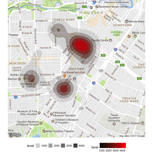
These 4 hotspots are located in:
- From Bagby St to San Jacinto St. via Webster St (The Heart of Midtown)
- Around San Jacinto and Eagle St (Reference: Fiesta Mart)
- Sul Ross St and Yupon St (Reference: University of St. Thomas Area)
- Cleveland St and Gillete St (Reference: Carnegie Vanguard High School)
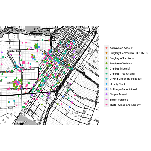
Midtown crime data points using geom_point()
Even though this visualization is not very intuitive, we can identify the density using the real crime incidents by incident type.
MidtownMap<-qmap("midtown houston",zoom=14,maptype="toner",
                    source="stamen",legend="right")

MidtownMap+
        geom_point(
                aes(x=longitude,y=latitude,colour=incident_type_primary),
                size=2,data=midtown
        )+theme(legend.title = element_blank())
All time Midtown hotspots by day of week
We can clearly see that the density is higher on Mondays for the heart of midtown area. However, looks like it is more likely to be affected by crime at the Fiesta Mart area on Thursdays. And the St. Thomas University Area is more dangerous on Tuesday.
MidtownMap<-qmap(location="midtown houston",zoom=14,legend="bottom")
MidtownMap+
        stat_density2d(
                aes(x=longitude,y=latitude, fill=..level..,alpha= ..level..),
                size=2,bins=6,data=midtown,
                geom="polygon"
        )+
        scale_fill_gradient(low="black",high="red")+
        facet_wrap(~ day_of_week)
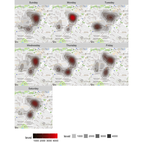
Of course, this is all time data, meaning that the temporal information may change over time, it does not necessarily represent the current density. We should take into account temporal patterns. Also, we need to consider more details, like type of incidents that are more likely to happen at certain times of the day than others.
To be continued…
I’ll update this post with an exploratory analysis by time of the day, last 2 years, last 5 years and see how these hotspots change. Also, we’ll discuss the type of crime within these hotspots by hour, day of the week and month. There are many ways to visualize crime.
References
There are many resources and posts out there that are vital to understand R and Crime analysis. You can find below all the references used in this post.
How to deal with date and time in R
Visualising Crime Hotspots in England and Wales using ggmap
ggmap: Spatial Visualization with ggplot2
Aggregating and analyzing data with dplyr
Kahle & Wikcham. (2013). “ggmap: Spatial Visualization with ggplot2”. The R Journal, Vol 5